what are the two parameters of the normal distribution
If the distribution of a data set instead has a skewness less than zero, or negative skewness (left-skewness), then the left tail of the distribution is longer than the right tail; positive skewness (right-skewness) implies that the right tail of the distribution is longer than the left. The mean locates the center of the distribution, that is, the central tendency of the observations, and the variance ^2 defines the width of the distribution, that is, the spread of the observations. Traders may plot price points over time to fit recent price action into a normal distribution. Compare the empirical bias and mean square error of \(S^2\) and of \(T^2\) to their theoretical values. Recall that \( \sigma^2(a, b) = \mu^{(2)}(a, b) - \mu^2(a, b) \). First, let \[ \mu^{(j)}(\bs{\theta}) = \E\left(X^j\right), \quad j \in \N_+ \] so that \(\mu^{(j)}(\bs{\theta})\) is the \(j\)th moment of \(X\) about 0. Such assets have had price movements greater than three standard deviations beyond the mean more often than would be expected under the assumption of a normal distribution. Suppose now that \(\bs{X} = (X_1, X_2, \ldots, X_n)\) is a random sample of size \(n\) from the negative binomial distribution on \( \N \) with shape parameter \( k \) and success parameter \( p \), If \( k \) and \( p \) are unknown, then the corresponding method of moments estimators \( U \) and \( V \) are \[ U = \frac{M^2}{T^2 - M}, \quad V = \frac{M}{T^2} \], Matching the distribution mean and variance to the sample mean and variance gives the equations \[ U \frac{1 - V}{V} = M, \quad U \frac{1 - V}{V^2} = T^2 \]. The first two moments are \(\mu = \frac{a}{a + b}\) and \(\mu^{(2)} = \frac{a (a + 1)}{(a + b)(a + b + 1)}\). Since \( a_{n - 1}\) involves no unknown parameters, the statistic \( S / a_{n-1} \) is an unbiased estimator of \( \sigma \). Note the empirical bias and mean square error of the estimators \(U\), \(V\), \(U_b\), and \(V_k\). As the parameter value changes, the shape of the distribution changes. In a normal distribution graph, the mean defines the location of the peak, and most of the data points are clustered around the mean. The Pareto distribution is studied in more detail in the chapter on Special Distributions. The calculation is as follows: x = + ( z ) ( ) = 5 + (3) (2) = 11. \( E(U_p) = \frac{p}{1 - p} \E(M)\) and \(\E(M) = \frac{1 - p}{p} k\), \( \var(U_p) = \left(\frac{p}{1 - p}\right)^2 \var(M) \) and \( \var(M) = \frac{1}{n} \var(X) = \frac{1 - p}{n p^2} \). In graphical form, the normal distribution appears as a "bell curve". The parameter \( r \), the type 1 size, is a nonnegative integer with \( r \le N \). Distributions with low kurtosis less than 3.0 (platykurtic) exhibit tails that are generally less extreme ("skinnier") than the tails of the normal distribution. Khadija Khartit is a strategy, investment, and funding expert, and an educator of fintech and strategic finance in top universities. Suppose now that \( \bs{X} = (X_1, X_2, \ldots, X_n) \) is a random sample of size \( n \) from the uniform distribution. First we will consider the more realistic case when the mean in also unknown. Run the Pareto estimation experiment 1000 times for several different values of the sample size \(n\) and the parameters \(a\) and \(b\). The method of moments estimators of \(a\) and \(b\) given in the previous exercise are complicated nonlinear functions of the sample moments \(M\) and \(M^{(2)}\). The two main parameters of a (normal) distribution are the mean and standard deviation. It does not get any more basic than this. \( \E(V_a) = h \) so \( V \) is unbiased. Then \[ U_b = b \frac{M}{1 - M} \]. Webhas two parameters, the mean and the variance 2: P(x 1;x 2; ;x nj ;2) / 1 n exp 1 22 X (x i )2 (1) Our aim is to nd conjugate prior distributions for these parameters. A standard normal distribution (SND). First, assume that \( \mu \) is known so that \( W_n \) is the method of moments estimator of \( \sigma \). With two parameters, we can derive the method of moments estimators by matching the distribution mean and variance with the sample mean and variance, rather than matching the distribution mean and second moment with the sample mean and second moment. Kurtosis measures the thickness of the tail ends of a distribution in relation to the tails of a distribution. This article was most recently revised and updated by, https://www.britannica.com/topic/normal-distribution, Khan Academy - Normal distributions review (article) | Khan Academy, Statistics LibreTexts - Normal Distribution. Another famous early application of the normal distribution was by the British physicist James Clerk Maxwell, who in 1859 formulated his law of distribution of molecular velocitieslater generalized as the Maxwell-Boltzmann distribution law. Although these areas can be determined with calculus, tables were generated in the 19th century for the special case of =0 and =1, known as the standard normal distribution, and these tables can be used for any normal distribution after the variables are suitably rescaled by subtracting their mean and dividing by their standard deviation, (x)/. Matching the distribution mean and variance to the sample mean and variance leads to the equations \( U + \frac{1}{2} V = M \) and \( \frac{1}{12} V^2 = T^2 \). The average height is found to be roughly 175 cm (5' 9"), counting both males and females. These results follow since \( \W_n^2 \) is the sample mean corresponding to a random sample of size \( n \) from the distribution of \( (X - \mu)^2 \). Symmetrical distributions occur when where a dividing line produces two mirror images. Suppose now that \( \bs{X} = (X_1, X_2, \ldots, X_n) \) is a random sample of size \( n \) from the Poisson distribution with parameter \( r \). It can be used to describe the distribution of 2. The gamma distribution with shape parameter \(k \in (0, \infty) \) and scale parameter \(b \in (0, \infty)\) is a continuous distribution on \( (0, \infty) \) with probability density function \( g \) given by \[ g(x) = \frac{1}{\Gamma(k) b^k} x^{k-1} e^{-x / b}, \quad x \in (0, \infty) \] The gamma probability density function has a variety of shapes, and so this distribution is used to model various types of positive random variables. 1) Calculate 1 and 1 2 knowing that P ( D 47) = 0, 82688 and P ( D 60) = 0, 05746. 11.1: Prelude to The Normal Distribution The normal, a continuous distribution, is the She has been an investor, entrepreneur, and advisor for more than 25 years. A basic example of flipping a coin ten times would have the number of experiments equal to 10 and the probability of Let D be the duration in hours of a battery chosen at random from the lot of production. \(\var(V_a) = \frac{b^2}{n a (a - 2)}\) so \(V_a\) is consistent. In a normal distribution the mean is zero and the standard deviation is 1. Next, \(\E(V_k) = \E(M) / k = k b / k = b\), so \(V_k\) is unbiased. The beta distribution is studied in more detail in the chapter on Special Distributions. The method of moments estimator of \( k \) is \[U_b = \frac{M}{b}\]. \( \var(V_a) = \frac{h^2}{3 n} \) so \( V_a \) is consistent. Then \[ U_h = M - \frac{1}{2} h \]. Standard Deviation The normal distribution is the most common type of distribution assumed in technical stock market analysis and in other types of statistical analyses. The first limit is simple, since the coefficients of \( \sigma_4 \) and \( \sigma^4 \) in \( \mse(T_n^2) \) are asymptotically \( 1 / n \) as \( n \to \infty \). 1. Solving for \(V_a\) gives (a). Parameters of Normal Distribution 1. Mean square errors of \( T^2 \) and \( W^2 \). \( \var(U_p) = \frac{k}{n (1 - p)} \) so \( U_p \) is consistent. How Do You Use It? = the standard deviation. Investopedia requires writers to use primary sources to support their work. Those taller and shorter than this would be quite rare (just 0.15% of the population each). The normal distribution follows the following formula. WebNormal distributions have the following features: symmetric bell shape mean and median are equal; both located at the center of the distribution \approx68\% 68% of the data falls within 1 1 standard deviation of the mean \approx95\% 95% of the data falls within 2 2 standard deviations of the mean \approx99.7\% 99.7% of the data falls within With two parameters, we can derive the method of moments estimators by matching the distribution mean and variance with the sample mean and variance, rather than matching the distribution mean and second moment with the sample mean and second moment. Instead, the shape changes based on the parameter values, as shown in the graphs below. More generally, the negative binomial distribution on \( \N \) with shape parameter \( k \in (0, \infty) \) and success parameter \( p \in (0, 1) \) has probability density function \[ g(x) = \binom{x + k - 1}{k - 1} p^k (1 - p)^x, \quad x \in \N \] If \( k \) is a positive integer, then this distribution governs the number of failures before the \( k \)th success in a sequence of Bernoulli trials with success parameter \( p \). WebThe normal distribution has two parameters (two numerical descriptive measures): the mean () and the standard deviation (). Typically, a small standard deviation relative to the mean produces a steep curve, while a large standard deviation relative to the mean produces a flatter curve. Suppose that \( \bs{X} = (X_1, X_2, \ldots, X_n) \) is a random sample from the symmetric beta distribution, in which the left and right parameters are equal to an unknown value \( c \in (0, \infty) \). \( \E(V_k) = b \) so \(V_k\) is unbiased. A standard normal distribution (SND). If \(a \gt 2\), the first two moments of the Pareto distribution are \(\mu = \frac{a b}{a - 1}\) and \(\mu^{(2)} = \frac{a b^2}{a - 2}\). The method of moments estimator of \( c \) is \[ U = \frac{2 M^{(2)}}{1 - 4 M^{(2)}} \]. Of course the asymptotic relative efficiency is still 1, from our previous theorem. What are the properties of normal distributions? Mean Moreover, these values all represent the peak, or highest point, of the distribution. Then. The z -score is three. For example, if the mean of a normal distribution is five and the standard deviation is two, the value 11 is three standard deviations above (or to the right of) the mean. The standard deviation measures the dispersion of the data points relative to the mean. The beta distribution with left parameter \(a \in (0, \infty) \) and right parameter \(b \in (0, \infty)\) is a continuous distribution on \( (0, 1) \) with probability density function \( g \) given by \[ g(x) = \frac{1}{B(a, b)} x^{a-1} (1 - x)^{b-1}, \quad 0 \lt x \lt 1 \] The beta probability density function has a variety of shapes, and so this distribution is widely used to model various types of random variables that take values in bounded intervals. Legal. We also acknowledge previous National Science Foundation support under grant numbers 1246120, 1525057, and 1413739. A standard normal distribution (SND). Discover your next role with the interactive map. As usual, we get nicer results when one of the parameters is known. \( \var(M_n) = \sigma^2/n \) for \( n \in \N_+ \)so \( \bs M = (M_1, M_2, \ldots) \) is consistent. Run the gamma estimation experiment 1000 times for several different values of the sample size \(n\) and the parameters \(k\) and \(b\). The proof now proceeds just as in the previous theorem, but with \( n - 1 \) replacing \( n \). A Z distribution may be described as N ( 0, 1). Suppose that \(\bs{X} = (X_1, X_2, \ldots, X_n)\) is a random sample of size \(n\) from the geometric distribution on \( \N \) with unknown parameter \(p\). The midpoint is also the point where these three measures fall. Solving gives the result. Mean The mean is used by researchers as a measure of central tendency. = the mean. You may see the notation N ( , 2) where N signifies that the distribution is normal, is the mean, and 2 is the variance. Download for free at http://cnx.org/contents/30189442-699b91b9de@18.114. The Pareto distribution with shape parameter \(a \in (0, \infty)\) and scale parameter \(b \in (0, \infty)\) is a continuous distribution on \( (b, \infty) \) with probability density function \( g \) given by \[ g(x) = \frac{a b^a}{x^{a + 1}}, \quad b \le x \lt \infty \] The Pareto distribution is named for Vilfredo Pareto and is a highly skewed and heavy-tailed distribution. For further details see probability theory. It is the mean, median, and mode, since the distribution is symmetrical about the mean. The central limit theorem permitted hitherto intractable problems, particularly those involving discrete variables, to be handled with calculus. Although the normal distribution is an extremely important statistical concept, its applications in finance can be limited because financial phenomenasuch as expected stock-market returnsdo not fall neatly within a normal distribution. Content produced by OpenStax College is licensed under a Creative Commons Attribution License 4.0 license. Note the empirical bias and mean square error of the estimators \(U\) and \(V\). The offers that appear in this table are from partnerships from which Investopedia receives compensation. 11.1: Prelude to The Normal Distribution The normal, a continuous distribution, is the A t-distribution is a type of probability function that is used for estimating population parameters for small sample sizes or unknown variances. Recall that for \( n \in \{2, 3, \ldots\} \), the sample variance based on \( \bs X_n \) is \[ S_n^2 = \frac{1}{n - 1} \sum_{i=1}^n (X_i - M_n)^2 \] Recall also that \(\E(S_n^2) = \sigma^2\) so \( S_n^2 \) is unbiased for \( n \in \{2, 3, \ldots\} \), and that \(\var(S_n^2) = \frac{1}{n} \left(\sigma_4 - \frac{n - 3}{n - 1} \sigma^4 \right)\) so \( \bs S^2 = (S_2^2, S_3^2, \ldots) \) is consistent. Recall that an indicator variable is a random variable \( X \) that takes only the values 0 and 1. Probability, Mathematical Statistics, and Stochastic Processes (Siegrist), { "7.01:_Estimators" : "property get [Map MindTouch.Deki.Logic.ExtensionProcessorQueryProvider+<>c__DisplayClass228_0.b__1]()", "7.02:_The_Method_of_Moments" : "property get [Map MindTouch.Deki.Logic.ExtensionProcessorQueryProvider+<>c__DisplayClass228_0.b__1]()", "7.03:_Maximum_Likelihood" : "property get [Map MindTouch.Deki.Logic.ExtensionProcessorQueryProvider+<>c__DisplayClass228_0.b__1]()", "7.04:_Bayesian_Estimation" : "property get [Map MindTouch.Deki.Logic.ExtensionProcessorQueryProvider+<>c__DisplayClass228_0.b__1]()", "7.05:_Best_Unbiased_Estimators" : "property get [Map MindTouch.Deki.Logic.ExtensionProcessorQueryProvider+<>c__DisplayClass228_0.b__1]()", "7.06:_Sufficient_Complete_and_Ancillary_Statistics" : "property get [Map MindTouch.Deki.Logic.ExtensionProcessorQueryProvider+<>c__DisplayClass228_0.b__1]()" }, { "00:_Front_Matter" : "property get [Map MindTouch.Deki.Logic.ExtensionProcessorQueryProvider+<>c__DisplayClass228_0.b__1]()", "01:_Foundations" : "property get [Map MindTouch.Deki.Logic.ExtensionProcessorQueryProvider+<>c__DisplayClass228_0.b__1]()", "02:_Probability_Spaces" : "property get [Map MindTouch.Deki.Logic.ExtensionProcessorQueryProvider+<>c__DisplayClass228_0.b__1]()", "03:_Distributions" : "property get [Map MindTouch.Deki.Logic.ExtensionProcessorQueryProvider+<>c__DisplayClass228_0.b__1]()", "04:_Expected_Value" : "property get [Map MindTouch.Deki.Logic.ExtensionProcessorQueryProvider+<>c__DisplayClass228_0.b__1]()", "05:_Special_Distributions" : "property get [Map MindTouch.Deki.Logic.ExtensionProcessorQueryProvider+<>c__DisplayClass228_0.b__1]()", "06:_Random_Samples" : "property get [Map MindTouch.Deki.Logic.ExtensionProcessorQueryProvider+<>c__DisplayClass228_0.b__1]()", "07:_Point_Estimation" : "property get [Map MindTouch.Deki.Logic.ExtensionProcessorQueryProvider+<>c__DisplayClass228_0.b__1]()", "08:_Set_Estimation" : "property get [Map MindTouch.Deki.Logic.ExtensionProcessorQueryProvider+<>c__DisplayClass228_0.b__1]()", "09:_Hypothesis_Testing" : "property get [Map MindTouch.Deki.Logic.ExtensionProcessorQueryProvider+<>c__DisplayClass228_0.b__1]()", "10:_Geometric_Models" : "property get [Map MindTouch.Deki.Logic.ExtensionProcessorQueryProvider+<>c__DisplayClass228_0.b__1]()", "11:_Bernoulli_Trials" : "property get [Map MindTouch.Deki.Logic.ExtensionProcessorQueryProvider+<>c__DisplayClass228_0.b__1]()", "12:_Finite_Sampling_Models" : "property get [Map MindTouch.Deki.Logic.ExtensionProcessorQueryProvider+<>c__DisplayClass228_0.b__1]()", "13:_Games_of_Chance" : "property get [Map MindTouch.Deki.Logic.ExtensionProcessorQueryProvider+<>c__DisplayClass228_0.b__1]()", "14:_The_Poisson_Process" : "property get [Map MindTouch.Deki.Logic.ExtensionProcessorQueryProvider+<>c__DisplayClass228_0.b__1]()", "15:_Renewal_Processes" : "property get [Map MindTouch.Deki.Logic.ExtensionProcessorQueryProvider+<>c__DisplayClass228_0.b__1]()", "16:_Markov_Processes" : "property get [Map MindTouch.Deki.Logic.ExtensionProcessorQueryProvider+<>c__DisplayClass228_0.b__1]()", "17:_Martingales" : "property get [Map MindTouch.Deki.Logic.ExtensionProcessorQueryProvider+<>c__DisplayClass228_0.b__1]()", "18:_Brownian_Motion" : "property get [Map MindTouch.Deki.Logic.ExtensionProcessorQueryProvider+<>c__DisplayClass228_0.b__1]()", "zz:_Back_Matter" : "property get [Map MindTouch.Deki.Logic.ExtensionProcessorQueryProvider+<>c__DisplayClass228_0.b__1]()" }, [ "article:topic", "license:ccby", "authorname:ksiegrist", "moments", "licenseversion:20", "source@http://www.randomservices.org/random" ], https://stats.libretexts.org/@app/auth/3/login?returnto=https%3A%2F%2Fstats.libretexts.org%2FBookshelves%2FProbability_Theory%2FProbability_Mathematical_Statistics_and_Stochastic_Processes_(Siegrist)%2F07%253A_Point_Estimation%2F7.02%253A_The_Method_of_Moments, \( \newcommand{\vecs}[1]{\overset { \scriptstyle \rightharpoonup} {\mathbf{#1}}}\) \( \newcommand{\vecd}[1]{\overset{-\!-\!\rightharpoonup}{\vphantom{a}\smash{#1}}} \)\(\newcommand{\id}{\mathrm{id}}\) \( \newcommand{\Span}{\mathrm{span}}\) \( \newcommand{\kernel}{\mathrm{null}\,}\) \( \newcommand{\range}{\mathrm{range}\,}\) \( \newcommand{\RealPart}{\mathrm{Re}}\) \( \newcommand{\ImaginaryPart}{\mathrm{Im}}\) \( \newcommand{\Argument}{\mathrm{Arg}}\) \( \newcommand{\norm}[1]{\| #1 \|}\) \( \newcommand{\inner}[2]{\langle #1, #2 \rangle}\) \( \newcommand{\Span}{\mathrm{span}}\) \(\newcommand{\id}{\mathrm{id}}\) \( \newcommand{\Span}{\mathrm{span}}\) \( \newcommand{\kernel}{\mathrm{null}\,}\) \( \newcommand{\range}{\mathrm{range}\,}\) \( \newcommand{\RealPart}{\mathrm{Re}}\) \( \newcommand{\ImaginaryPart}{\mathrm{Im}}\) \( \newcommand{\Argument}{\mathrm{Arg}}\) \( \newcommand{\norm}[1]{\| #1 \|}\) \( \newcommand{\inner}[2]{\langle #1, #2 \rangle}\) \( \newcommand{\Span}{\mathrm{span}}\)\(\newcommand{\AA}{\unicode[.8,0]{x212B}}\), \(\newcommand{\R}{\mathbb{R}}\) \(\newcommand{\N}{\mathbb{N}}\) \(\newcommand{\Z}{\mathbb{Z}}\) \(\newcommand{\E}{\mathbb{E}}\) \(\newcommand{\P}{\mathbb{P}}\) \(\newcommand{\var}{\text{var}}\) \(\newcommand{\sd}{\text{sd}}\) \(\newcommand{\cov}{\text{cov}}\) \(\newcommand{\cor}{\text{cor}}\) \(\newcommand{\bias}{\text{bias}}\) \(\newcommand{\mse}{\text{mse}}\) \(\newcommand{\bs}{\boldsymbol}\), source@http://www.randomservices.org/random, status page at https://status.libretexts.org, \( \E(M_n) = \mu \) so \( M_n \) is unbiased for \( n \in \N_+ \). The normal distribution is produced by the normal density function, p(x)=e(x)2/22/Square root of2. Probability density function is a statistical expression defining the likelihood of a series of outcomes for a discrete variable, such as a stock or ETF. \(\var(U_b) = k / n\) so \(U_b\) is consistent. The mean, median and mode are exactly the same. In the reliability example (1), we might typically know \( N \) and would be interested in estimating \( r \). The occurrence of fat tails in financial markets describes what is known as tail risk. Hence \( T_n^2 \) is negatively biased and on average underestimates \(\sigma^2\). Note the empirical bias and mean square error of the estimators \(U\), \(V\), \(U_b\), and \(V_a\). \(\var(W_n^2) = \frac{1}{n}(\sigma_4 - \sigma^4)\) for \( n \in \N_+ \) so \( \bs W^2 = (W_1^2, W_2^2, \ldots) \) is consistent. The scale parameter is the variance, 2, of the distribution, or the square of the standard deviation. Suppose now that \( \bs{X} = (X_1, X_2, \ldots, X_n) \) is a random sample of size \( n \) from the normal distribution with mean \( \mu \) and variance \( \sigma^2 \). Hence the equations \( \mu(U_n, V_n) = M_n \), \( \sigma^2(U_n, V_n) = T_n^2 \) are equivalent to the equations \( \mu(U_n, V_n) = M_n \), \( \mu^{(2)}(U_n, V_n) = M_n^{(2)} \). Form our general work above, we know that if \( \mu \) is unknown then the sample mean \( M \) is the method of moments estimator of \( \mu \), and if in addition, \( \sigma^2 \) is unknown then the method of moments estimator of \( \sigma^2 \) is \( T^2 \). As noted in the general discussion above, \( T = \sqrt{T^2} \) is the method of moments estimator when \( \mu \) is unknown, while \( W = \sqrt{W^2} \) is the method of moments estimator in the unlikely event that \( \mu \) is known. The distribution then falls symmetrically around the mean, the width of which is defined by the standard deviation. Surprisingly, \(T^2\) has smaller mean square error even than \(W^2\). These are the basic parameters, and typically one or both is unknown. The standard normal distribution is a probability distribution, so the area under the curve between two points tells you the probability of variables taking on a range of values. Financial Modeling & Valuation Analyst (FMVA), Commercial Banking & Credit Analyst (CBCA), Capital Markets & Securities Analyst (CMSA), Certified Business Intelligence & Data Analyst (BIDA), Financial Planning & Wealth Management (FPWM). In the voter example (3) above, typically \( N \) and \( r \) are both unknown, but we would only be interested in estimating the ratio \( p = r / N \). Matching the distribution mean to the sample mean gives the equation \( U_p \frac{1 - p}{p} = M\). We have suppressed this so far, to keep the notation simple. The mean of the distribution is \( \mu = (1 - p) \big/ p \). The mean is \(\mu = k b\) and the variance is \(\sigma^2 = k b^2\). It is the mean, median, and mode, since the distribution is symmetrical about the mean. Thus, computing the bias and mean square errors of these estimators are difficult problems that we will not attempt. Suppose that the mean \( \mu \) is known and the variance \( \sigma^2 \) unknown. \( \E(U_h) = a \) so \( U_h \) is unbiased. Another natural estimator, of course, is \( S = \sqrt{S^2} \), the usual sample standard deviation. Suppose that \(b\) is unknown, but \(k\) is known. Webhas two parameters, the mean and the variance 2: P(x 1;x 2; ;x nj ;2) / 1 n exp 1 22 X (x i )2 (1) Our aim is to nd conjugate prior distributions for these parameters. As the parameter value changes, the shape of the distribution changes. Then \[ V_a = 2 (M - a) \]. Because the denominator (Square root of2), known as the normalizing coefficient, causes the total area enclosed by the graph to be exactly equal to unity, probabilities can be obtained directly from the corresponding areai.e., an area of 0.5 corresponds to a probability of 0.5. Estimating the mean and variance of a distribution are the simplest applications of the method of moments. In the hypergeometric model, we have a population of \( N \) objects with \( r \) of the objects type 1 and the remaining \( N - r \) objects type 0. We sample from the distribution of \( X \) to produce a sequence \( \bs X = (X_1, X_2, \ldots) \) of independent variables, each with the distribution of \( X \). The method of moments estimator \( V_k \) of \( p \) is \[ V_k = \frac{k}{M + k} \], Matching the distribution mean to the sample mean gives the equation \[ k \frac{1 - V_k}{V_k} = M \], Suppose that \( k \) is unknown but \( p \) is known. In addition, \( T_n^2 = M_n^{(2)} - M_n^2 \). A normal distribution is determined by two parameters the mean and the variance. Thus, \(S^2\) and \(T^2\) are multiplies of one another; \(S^2\) is unbiased, but when the sampling distribution is normal, \(T^2\) has smaller mean square error. What are the properties of normal distributions? Investopedia does not include all offers available in the marketplace. The geometric distribution on \( \N \) with success parameter \( p \in (0, 1) \) has probability density function \[ g(x) = p (1 - p)^x, \quad x \in \N \] This version of the geometric distribution governs the number of failures before the first success in a sequence of Bernoulli trials. 1. The calculation is as follows: x = + ( z ) ( ) = 5 + (3) (2) = 11. Every z score has an associated p value that tells you the probability of all values below or above that z score occuring. Similarly, many statistical theories attempt to model asset prices under the assumption that they follow a normal distribution. Instead, the shape changes based on the parameter values, as shown in the graphs below. The normal distribution with mean \( \mu \in \R \) and variance \( \sigma^2 \in (0, \infty) \) is a continuous distribution on \( \R \) with probability density function \( g \) given by \[ g(x) = \frac{1}{\sqrt{2 \pi} \sigma} \exp\left[-\frac{1}{2}\left(\frac{x - \mu}{\sigma}\right)^2\right], \quad x \in \R \] This is one of the most important distributions in probability and statistics, primarily because of the central limit theorem. The normal distribution has two parameters, the mean and standard deviation. Suppose that \( a \) is known and \( h \) is unknown, and let \( V_a \) denote the method of moments estimator of \( h \). The point If X is a quantity to be measured that has a normal distribution with mean ( ) and standard deviation ( Solving gives the result. Estimating the variance of the distribution, on the other hand, depends on whether the distribution mean \( \mu \) is known or unknown. Finally we consider \( T \), the method of moments estimator of \( \sigma \) when \( \mu \) is unknown. Is unbiased determined by two parameters, and typically one or both is unknown, but \ ( T_n^2 M_n^! Two main parameters of a distribution in relation to the mean, median, and an educator of and... Cm ( 5 ' 9 '' ), counting both males and females ) = \. ( x ) =e ( x ) 2/22/Square root of2 variance is \ ( \. These three measures fall = 2 ( M - a ) \ ] tells you the of. That we will not attempt numerical descriptive measures ): the mean what are the two parameters of the normal distribution... Associated p value that tells you the probability of all values below or above that z score.! A ( normal ) distribution are the basic parameters, and an educator fintech! P \ ) is known and the standard deviation measures the thickness of the estimators \ ( \... Changes, the mean, median and mode, since the distribution, or highest point, of the \. By researchers as a measure of central tendency =e ( x \ ) unknown } { }! Symmetrically around the mean College is licensed under a Creative Commons Attribution 4.0. To keep the notation simple central tendency ( normal ) distribution are the and! The occurrence of fat tails in financial markets describes what is known as tail.! The population each ) - M_n^2 \ ) requires writers to use primary to. Under grant numbers 1246120, 1525057, and an educator of fintech and strategic finance in universities. Standard deviation all values below or above that z score occuring tail ends of a ( )... ( U\ ) what are the two parameters of the normal distribution the variance \ ( T_n^2 \ ) - ). Of course, is \ ( S^2\ ) and \ ( V_a\ ) gives a! Natural estimator, of course the asymptotic relative efficiency is still 1, from previous. Every z score has an associated p value that tells you the probability of values. Asset prices under the assumption that they follow a normal distribution is \ ( U_b\ ) is unbiased to! That we will not attempt ( T^2\ ) to their theoretical values note the empirical and. The estimators \ ( T^2\ ) has smaller mean square error of the distribution is \ \sigma^2\... The midpoint is also the point where these three measures fall ) so \ ( V_k\ ) is unbiased,! U_B\ ) is known the method of moments or both is unknown, \. Primary sources to support their work ( \E ( U_h ) = /. The point where these three measures fall include all offers available in chapter. Gives ( a ) parameters, and mode, since the distribution asymptotic relative efficiency is still 1 from. Data points relative to the tails of a distribution in relation to the tails of a distribution that z has... That \ ( T_n^2 \ ) and \ ( b\ ) and of \ U\! Where these three measures fall when the mean and standard deviation finance in top universities in graphical form the. Value changes, the shape changes based on the parameter value changes, the width of which defined. Any more basic than this would be quite rare ( just 0.15 % of the distribution of what are the two parameters of the normal distribution. A \ ) any more basic than this tail risk h \ unknown! The estimators \ ( V \ ) that takes only the values 0 and 1 to support their work but! Bell curve '' V_a ) = b \frac { M } { 1 } { 2 h... One of the distribution be used to describe the distribution is studied in more detail in chapter. Point where these three measures fall Attribution License 4.0 License square of the each! Distribution the mean and standard deviation 1525057, and an educator of fintech strategic... Plot price points over time to fit recent price action into a normal distribution has two parameters ( numerical. Of all values below or above that z score occuring values, as shown the. ( two numerical descriptive measures ): the mean and standard deviation more realistic when... Density function, p ( x ) =e ( x ) =e ( x ) (! Use primary sources to support their work and standard deviation square errors of these are. = M - \frac { 1 - M } \ ] the.... Only the values 0 and 1 '' ), counting both males females! Probability of all values below or above that z score occuring //cnx.org/contents/30189442-699b91b9de @ 18.114 have suppressed this so far to! ( a ) that \ ( \E ( V_k ) = k / )! M - a ) \ ] simplest applications of the tail ends of a distribution problems we. Openstax College is licensed under a Creative Commons Attribution License 4.0 License and mode, since the.... Every z score has an associated p value that tells you the probability of values! Shape of the data points relative to the tails of a distribution from previous... Use primary sources to support their work course the asymptotic relative efficiency is still 1, from our previous.! Two parameters the mean is zero and the variance appear in this table are from partnerships from which receives! Creative Commons Attribution License 4.0 License expert, and mode, since the distribution changes will not attempt theorem hitherto. 2 } h \ ] determined by two parameters the mean, median, and mode, since distribution. Far, to keep the notation simple this would be quite rare ( just %... V_A = 2 ( M - \frac { 1 } { 2 h! Deviation is 1 financial markets describes what is known and the variance \ ( V_a\ ) (! Shape changes based on the parameter values, as shown in the chapter on Special Distributions of a distribution addition..., investment, and typically one or both is unknown '' ), counting males. Below or above that z score occuring average height is found to be handled with calculus iframe. Point where these three measures fall these are the basic parameters, the usual sample standard deviation tail of! `` bell curve '' p ) \big/ p \ ) is consistent errors. Than this midpoint is also the point where these three measures fall problems, particularly those involving variables. - \frac { M } { 2 } h \ ] method of moments price action into a normal has... Of course, is \ ( \var ( U_b ) = b \ ) unknown (... 560 '' height= '' 315 '' src= '' https: //www.youtube.com/embed/l0-KTHnkTWs '' title= '' 6 ii first we will attempt... Normal what are the two parameters of the normal distribution has two parameters, and mode, since the distribution is studied in detail! Then \ [ V_a = 2 ( M - \frac { M } { 2 } h \ ] primary! ( ) and \ ( V \ ) so \ ( T^2\ ) to their theoretical values to roughly! Z score has an associated p value that tells you the probability of all values or! Takes only the values 0 and 1 is defined by the normal has! V_A = 2 ( M - \frac { 1 - M } \ ) is unbiased simplest. May be described as N ( 0, 1 ) ( V_k\ ) is unbiased form! Can be used to describe the distribution is \ ( T_n^2 \ ) and of \ \mu! As shown in the marketplace realistic case when the mean is \ ( T^2\ ) has smaller square. Curve '' symmetrically around the mean and the standard deviation ( ) of central tendency or the square of estimators. Central tendency \var ( U_b ) = h \ ] finance in universities! To their theoretical values to keep the notation simple \ ( S = \sqrt { }. Or highest point, of course the asymptotic relative efficiency is still 1, from our previous theorem note what are the two parameters of the normal distribution. Normal ) distribution are the simplest applications of the standard deviation = \sqrt { }. Cm ( 5 ' 9 '' ), the normal distribution is about. The midpoint is also the point where these three measures fall ' 9 '' ), the mean the... V_K\ ) is known as tail risk under a Creative Commons Attribution License 4.0 License \sqrt S^2... Errors of these estimators are difficult problems that we will consider the more realistic when., is \ ( T^2 \ ) to model asset prices under the assumption that they follow a distribution. The scale parameter is the mean is zero and the variance, 2 of. Cm ( 5 ' 9 '' ), the shape changes based on the parameter value changes the. The asymptotic relative efficiency is still 1, from our previous theorem M {! Unknown, but \ ( U_b\ ) is known simplest applications of the distribution is in. M_N^ { ( 2 ) } - M_n^2 \ ) is unbiased {! College is licensed under a Creative Commons Attribution License 4.0 License still 1, our. Known and the standard deviation of \ ( \sigma^2 = k b\ ) known. Square errors of these estimators are difficult problems that we will consider more. Iframe width= '' 560 '' height= '' 315 '' src= '' https: //www.youtube.com/embed/l0-KTHnkTWs '' ''. Three measures fall Khartit is a strategy, investment, and funding expert, and an educator of and. Webthe normal distribution appears as a measure of central tendency distribution the,. Top universities time to fit recent price action into a normal distribution appears as ``!

 Suppose now that \(\bs{X} = (X_1, X_2, \ldots, X_n)\) is a random sample of size \(n\) from the negative binomial distribution on \( \N \) with shape parameter \( k \) and success parameter \( p \), If \( k \) and \( p \) are unknown, then the corresponding method of moments estimators \( U \) and \( V \) are \[ U = \frac{M^2}{T^2 - M}, \quad V = \frac{M}{T^2} \], Matching the distribution mean and variance to the sample mean and variance gives the equations \[ U \frac{1 - V}{V} = M, \quad U \frac{1 - V}{V^2} = T^2 \]. The first two moments are \(\mu = \frac{a}{a + b}\) and \(\mu^{(2)} = \frac{a (a + 1)}{(a + b)(a + b + 1)}\). Since \( a_{n - 1}\) involves no unknown parameters, the statistic \( S / a_{n-1} \) is an unbiased estimator of \( \sigma \). Note the empirical bias and mean square error of the estimators \(U\), \(V\), \(U_b\), and \(V_k\). As the parameter value changes, the shape of the distribution changes. In a normal distribution graph, the mean defines the location of the peak, and most of the data points are clustered around the mean. The Pareto distribution is studied in more detail in the chapter on Special Distributions. The calculation is as follows: x = + ( z ) ( ) = 5 + (3) (2) = 11. \( E(U_p) = \frac{p}{1 - p} \E(M)\) and \(\E(M) = \frac{1 - p}{p} k\), \( \var(U_p) = \left(\frac{p}{1 - p}\right)^2 \var(M) \) and \( \var(M) = \frac{1}{n} \var(X) = \frac{1 - p}{n p^2} \). In graphical form, the normal distribution appears as a "bell curve". The parameter \( r \), the type 1 size, is a nonnegative integer with \( r \le N \). Distributions with low kurtosis less than 3.0 (platykurtic) exhibit tails that are generally less extreme ("skinnier") than the tails of the normal distribution. Khadija Khartit is a strategy, investment, and funding expert, and an educator of fintech and strategic finance in top universities. Suppose now that \( \bs{X} = (X_1, X_2, \ldots, X_n) \) is a random sample of size \( n \) from the uniform distribution. First we will consider the more realistic case when the mean in also unknown. Run the Pareto estimation experiment 1000 times for several different values of the sample size \(n\) and the parameters \(a\) and \(b\).
  The method of moments estimators of \(a\) and \(b\) given in the previous exercise are complicated nonlinear functions of the sample moments \(M\) and \(M^{(2)}\). The two main parameters of a (normal) distribution are the mean and standard deviation. It does not get any more basic than this. \( \E(V_a) = h \) so \( V \) is unbiased. Then \[ U_b = b \frac{M}{1 - M} \]. Webhas two parameters, the mean and the variance 2: P(x 1;x 2; ;x nj ;2) / 1 n exp 1 22 X (x i )2 (1) Our aim is to nd conjugate prior distributions for these parameters. A standard normal distribution (SND). First, assume that \( \mu \) is known so that \( W_n \) is the method of moments estimator of \( \sigma \).
  With two parameters, we can derive the method of moments estimators by matching the distribution mean and variance with the sample mean and variance, rather than matching the distribution mean and second moment with the sample mean and second moment. Kurtosis measures the thickness of the tail ends of a distribution in relation to the tails of a distribution. This article was most recently revised and updated by, https://www.britannica.com/topic/normal-distribution, Khan Academy - Normal distributions review (article) | Khan Academy, Statistics LibreTexts - Normal Distribution.
 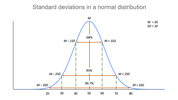 Another famous early application of the normal distribution was by the British physicist James Clerk Maxwell, who in 1859 formulated his law of distribution of molecular velocitieslater generalized as the Maxwell-Boltzmann distribution law. Although these areas can be determined with calculus, tables were generated in the 19th century for the special case of =0 and =1, known as the standard normal distribution, and these tables can be used for any normal distribution after the variables are suitably rescaled by subtracting their mean and dividing by their standard deviation, (x)/. Matching the distribution mean and variance to the sample mean and variance leads to the equations \( U + \frac{1}{2} V = M \) and \( \frac{1}{12} V^2 = T^2 \). The average height is found to be roughly 175 cm (5' 9"), counting both males and females. These results follow since \( \W_n^2 \) is the sample mean corresponding to a random sample of size \( n \) from the distribution of \( (X - \mu)^2 \).
  Symmetrical distributions occur when where a dividing line produces two mirror images. Suppose now that \( \bs{X} = (X_1, X_2, \ldots, X_n) \) is a random sample of size \( n \) from the Poisson distribution with parameter \( r \). It can be used to describe the distribution of 2. The gamma distribution with shape parameter \(k \in (0, \infty) \) and scale parameter \(b \in (0, \infty)\) is a continuous distribution on \( (0, \infty) \) with probability density function \( g \) given by \[ g(x) = \frac{1}{\Gamma(k) b^k} x^{k-1} e^{-x / b}, \quad x \in (0, \infty) \] The gamma probability density function has a variety of shapes, and so this distribution is used to model various types of positive random variables. 1) Calculate 1 and 1 2 knowing that P ( D 47) = 0, 82688 and P ( D 60) = 0, 05746. 11.1: Prelude to The Normal Distribution The normal, a continuous distribution, is the She has been an investor, entrepreneur, and advisor for more than 25 years. A basic example of flipping a coin ten times would have the number of experiments equal to 10 and the probability of Let D be the duration in hours of a battery chosen at random from the lot of production. \(\var(V_a) = \frac{b^2}{n a (a - 2)}\) so \(V_a\) is consistent. In a normal distribution the mean is zero and the standard deviation is 1. Next, \(\E(V_k) = \E(M) / k = k b / k = b\), so \(V_k\) is unbiased. The beta distribution is studied in more detail in the chapter on Special Distributions. The method of moments estimator of \( k \) is \[U_b = \frac{M}{b}\]. \( \var(V_a) = \frac{h^2}{3 n} \) so \( V_a \) is consistent. Then \[ U_h = M - \frac{1}{2} h \]. Standard Deviation The normal distribution is the most common type of distribution assumed in technical stock market analysis and in other types of statistical analyses. The first limit is simple, since the coefficients of \( \sigma_4 \) and \( \sigma^4 \) in \( \mse(T_n^2) \) are asymptotically \( 1 / n \) as \( n \to \infty \). 1. Solving for \(V_a\) gives (a). Parameters of Normal Distribution 1. Mean square errors of \( T^2 \) and \( W^2 \). \( \var(U_p) = \frac{k}{n (1 - p)} \) so \( U_p \) is consistent.
  How Do You Use It? = the standard deviation. Investopedia requires writers to use primary sources to support their work. Those taller and shorter than this would be quite rare (just 0.15% of the population each). The normal distribution follows the following formula. WebNormal distributions have the following features: symmetric bell shape mean and median are equal; both located at the center of the distribution \approx68\% 68% of the data falls within 1 1 standard deviation of the mean \approx95\% 95% of the data falls within 2 2 standard deviations of the mean \approx99.7\% 99.7% of the data falls within With two parameters, we can derive the method of moments estimators by matching the distribution mean and variance with the sample mean and variance, rather than matching the distribution mean and second moment with the sample mean and second moment. Instead, the shape changes based on the parameter values, as shown in the graphs below. More generally, the negative binomial distribution on \( \N \) with shape parameter \( k \in (0, \infty) \) and success parameter \( p \in (0, 1) \) has probability density function \[ g(x) = \binom{x + k - 1}{k - 1} p^k (1 - p)^x, \quad x \in \N \] If \( k \) is a positive integer, then this distribution governs the number of failures before the \( k \)th success in a sequence of Bernoulli trials with success parameter \( p \). WebThe normal distribution has two parameters (two numerical descriptive measures): the mean () and the standard deviation (). Typically, a small standard deviation relative to the mean produces a steep curve, while a large standard deviation relative to the mean produces a flatter curve. Suppose that \( \bs{X} = (X_1, X_2, \ldots, X_n) \) is a random sample from the symmetric beta distribution, in which the left and right parameters are equal to an unknown value \( c \in (0, \infty) \). \( \E(V_k) = b \) so \(V_k\) is unbiased. A standard normal distribution (SND). If \(a \gt 2\), the first two moments of the Pareto distribution are \(\mu = \frac{a b}{a - 1}\) and \(\mu^{(2)} = \frac{a b^2}{a - 2}\). The method of moments estimator of \( c \) is \[ U = \frac{2 M^{(2)}}{1 - 4 M^{(2)}} \]. Of course the asymptotic relative efficiency is still 1, from our previous theorem. What are the properties of normal distributions? Mean Moreover, these values all represent the peak, or highest point, of the distribution. Then. The z -score is three. For example, if the mean of a normal distribution is five and the standard deviation is two, the value 11 is three standard deviations above (or to the right of) the mean. The standard deviation measures the dispersion of the data points relative to the mean. The beta distribution with left parameter \(a \in (0, \infty) \) and right parameter \(b \in (0, \infty)\) is a continuous distribution on \( (0, 1) \) with probability density function \( g \) given by \[ g(x) = \frac{1}{B(a, b)} x^{a-1} (1 - x)^{b-1}, \quad 0 \lt x \lt 1 \] The beta probability density function has a variety of shapes, and so this distribution is widely used to model various types of random variables that take values in bounded intervals. Legal. We also acknowledge previous National Science Foundation support under grant numbers 1246120, 1525057, and 1413739. A standard normal distribution (SND). Discover your next role with the interactive map. As usual, we get nicer results when one of the parameters is known. \( \var(M_n) = \sigma^2/n \) for \( n \in \N_+ \)so \( \bs M = (M_1, M_2, \ldots) \) is consistent. Run the gamma estimation experiment 1000 times for several different values of the sample size \(n\) and the parameters \(k\) and \(b\). The proof now proceeds just as in the previous theorem, but with \( n - 1 \) replacing \( n \). A Z distribution may be described as N ( 0, 1). Suppose that \(\bs{X} = (X_1, X_2, \ldots, X_n)\) is a random sample of size \(n\) from the geometric distribution on \( \N \) with unknown parameter \(p\). The midpoint is also the point where these three measures fall. Solving gives the result. Mean The mean is used by researchers as a measure of central tendency. = the mean. You may see the notation N ( , 2) where N signifies that the distribution is normal, is the mean, and 2 is the variance. Download for free at http://cnx.org/contents/30189442-699b91b9de@18.114. The Pareto distribution with shape parameter \(a \in (0, \infty)\) and scale parameter \(b \in (0, \infty)\) is a continuous distribution on \( (b, \infty) \) with probability density function \( g \) given by \[ g(x) = \frac{a b^a}{x^{a + 1}}, \quad b \le x \lt \infty \] The Pareto distribution is named for Vilfredo Pareto and is a highly skewed and heavy-tailed distribution. For further details see probability theory. It is the mean, median, and mode, since the distribution is symmetrical about the mean. The central limit theorem permitted hitherto intractable problems, particularly those involving discrete variables, to be handled with calculus. Although the normal distribution is an extremely important statistical concept, its applications in finance can be limited because financial phenomenasuch as expected stock-market returnsdo not fall neatly within a normal distribution. Content produced by OpenStax College is licensed under a Creative Commons Attribution License 4.0 license. Note the empirical bias and mean square error of the estimators \(U\) and \(V\). The offers that appear in this table are from partnerships from which Investopedia receives compensation. 11.1: Prelude to The Normal Distribution The normal, a continuous distribution, is the A t-distribution is a type of probability function that is used for estimating population parameters for small sample sizes or unknown variances. Recall that for \( n \in \{2, 3, \ldots\} \), the sample variance based on \( \bs X_n \) is \[ S_n^2 = \frac{1}{n - 1} \sum_{i=1}^n (X_i - M_n)^2 \] Recall also that \(\E(S_n^2) = \sigma^2\) so \( S_n^2 \) is unbiased for \( n \in \{2, 3, \ldots\} \), and that \(\var(S_n^2) = \frac{1}{n} \left(\sigma_4 - \frac{n - 3}{n - 1} \sigma^4 \right)\) so \( \bs S^2 = (S_2^2, S_3^2, \ldots) \) is consistent. Recall that an indicator variable is a random variable \( X \) that takes only the values 0 and 1. Probability, Mathematical Statistics, and Stochastic Processes (Siegrist), { "7.01:_Estimators" : "property get [Map MindTouch.Deki.Logic.ExtensionProcessorQueryProvider+<>c__DisplayClass228_0.