
s ) -plane, s 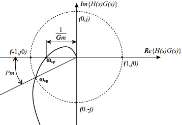 N We know from Figure \(\PageIndex{3}\) that this case of \(\Lambda=4.75\) is closed-loop unstable. ( You can achieve greater accuracy using it. ( Conclusions can also be reached by examining the open loop transfer function (OLTF) who played aunt ruby in madea's family reunion; nami dupage support groups; WebNyquist plot of the transfer function s/(s-1)^3. Natural Language; Math Input; Extended Keyboard Examples Upload Random. Is the open loop system stable? I'm glad that this tool is being used, in any case! + I learned about this in ELEC 341, the systems and controls class. F G ) Let us continue this study by computing \(OLFRF(\omega)\) and displaying it as a Nyquist plot for an intermediate value of gain, \(\Lambda=4.75\), for which Figure \(\PageIndex{3}\) shows the closed-loop system is unstable. Nevertheless, there are generalizations of the Nyquist criterion (and plot) for non-linear systems, such as the circle criterion and the scaled relative graph of a nonlinear operator. 1 charles city death notices. The feedback loop has stabilized the unstable open loop systems with \(-1 < a \le 0\). For example, audio CDs have a sampling rate of 44100 samples/second. G There are two poles in the right half-plane, so the open loop system \(G(s)\) is unstable. Let \(\gamma_R = C_1 + C_R\). = +
  Section 17.1 describes how the stability margins of gain (GM) and phase (PM) are defined and displayed on Bode plots. \(\PageIndex{4}\) includes the Nyquist plots for both \(\Lambda=0.7\) and \(\Lambda =\Lambda_{n s 1}\), the latter of which by definition crosses the negative \(\operatorname{Re}[O L F R F]\) axis at the point \(-1+j 0\), not far to the left of where the \(\Lambda=0.7\) plot crosses at about \(-0.73+j 0\); therefore, it might be that the appropriate value of gain margin for \(\Lambda=0.7\) is found from \(1 / \mathrm{GM}_{0.7} \approx 0.73\), so that \(\mathrm{GM}_{0.7} \approx 1.37=2.7\) dB, a small gain margin indicating that the closed-loop system is just weakly stable.
  charles city death notices. T ( Since the number of poles of \(G\) in the right half-plane is the same as this winding number, the closed loop system is stable. Closed Loop Transfer Function: Characteristic Equation: 1 + G c G v G p G m =0 (Note: This equation is not a polynomial but a ratio of polynomials) Stability Condition: None of the zeros of ( 1 + G c G v G p G m )are in the right half plane. {\displaystyle G(s)} The value of \(\Lambda_{n s 2}\) is not exactly 15, as Figure \(\PageIndex{3}\) might suggest; see homework Problem 17.2(b) for calculation of the more precise value \(\Lambda_{n s 2} = 15.0356\). Open the Nyquist Plot applet at. Let us begin this study by computing \(\operatorname{OLFRF}(\omega)\) and displaying it on Nyquist plots for a low value of gain, \(\Lambda=0.7\) (for which the closed-loop system is stable), and for the value corresponding to the transition from stability to instability on Figure \(\PageIndex{3}\), which we denote as \(\Lambda_{n s 1} \approx 1\). {\displaystyle N=P-Z} {\displaystyle 1+G(s)} ) ) j The Nyquist criterion is a graphical technique for telling whether an unstable linear time invariant system can be stabilized using a negative feedback loop. ) N r WebNyquist Stability Criterion It states that the number of unstable closed-looppoles is equal to the number of unstable open-looppoles plus the number of encirclements of the origin of the Nyquist plot of the complex function . WebThe Nyquist stability criterion covered in Section 11.2.2 is covering only SISO systems and this section is the extension for MIMO systems which is called the generalized Nyquist criterion (GNC). If the number of poles is greater than the number of zeros, then the Nyquist criterion tells us how to use the Nyquist plot to graphically determine the stability of the closed loop system. The Nyquist criterion gives a graphical method for checking the stability of the closed loop system. F N , that starts at Physically the modes tell us the behavior of the system when the input signal is 0, but there are initial conditions. + {\displaystyle -1/k} The answer is no, \(G_{CL}\) is not stable. However, to ensure robust stability and desirable circuit performance, the gain at f180 should be significantly less {\displaystyle F(s)} ) ) G This gives us, We now note that s a clockwise semicircle at L(s)= in "L(s)" (see, The clockwise semicircle at infinity in "s" corresponds to a single That is, the Nyquist plot is the image of the imaginary axis under the map \(w = kG(s)\). s s {\displaystyle G(s)} WebIn general each example has five sections: 1) A definition of the loop gain, 2) A Nyquist plot made by the NyquistGui program, 3) a Nyquist plot made by Matlab, 4) A discussion of the plots and system stability, and 5) a video of the output of the NyquistGui program. gain margin as defined on Figure \(\PageIndex{5}\) can be an ambiguous, unreliable, and even deceptive metric of closed-loop stability; phase margin as defined on Figure \(\PageIndex{5}\), on the other hand, is usually an unambiguous and reliable metric, with \(\mathrm{PM}>0\) indicating closed-loop stability, and \(\mathrm{PM}<0\) indicating closed-loop instability. ( While Nyquist is one of the most general stability tests, it is still restricted to linear, time-invariant (LTI) systems. Set the feedback factor \(k = 1\). These are the same systems as in the examples just above. s = I learned about this in ELEC 341, the systems and controls class. Accessibility StatementFor more information contact us atinfo@libretexts.orgor check out our status page at https://status.libretexts.org. 1 + WebSimple VGA core sim used in CPEN 311. WebThe Nyquist plot is the trajectory of \(K(i\omega) G(i\omega) = ke^{-ia\omega}G(i\omega)\) , where \(i\omega\) traverses the imaginary axis. ( WebSimple VGA core sim used in CPEN 311. ( In this case the winding number around -1 is 0 and the Nyquist criterion says the closed loop system is stable if and only if the open loop system is stable. = + The positive \(\mathrm{PM}_{\mathrm{S}}\) for a closed-loop-stable case is the counterclockwise angle from the negative \(\operatorname{Re}[O L F R F]\) axis to the intersection of the unit circle with the \(OLFRF_S\) curve; conversely, the negative \(\mathrm{PM}_U\) for a closed-loop-unstable case is the clockwise angle from the negative \(\operatorname{Re}[O L F R F]\) axis to the intersection of the unit circle with the \(OLFRF_U\) curve. The fundamental stability criterion is that the magnitude of the loop gain must be less than unity at f180. be the number of poles of enclosing the right half plane, with indentations as needed to avoid passing through zeros or poles of the function {\displaystyle G(s)} The Nyquist plot of . Since they are all in the left half-plane, the system is stable. I. {\displaystyle F(s)} However, the gain margin calculated from either of the two phase crossovers suggests instability, showing that both are deceptively defective metrics of stability. If, on the other hand, we were to calculate gain margin using the other phase crossing, at about \(-0.04+j 0\), then that would lead to the exaggerated \(\mathrm{GM} \approx 25=28\) dB, which is obviously a defective metric of stability. ( We regard this closed-loop system as being uncommon or unusual because it is stable for small and large values of gain \(\Lambda\), but unstable for a range of intermediate values. H and travels anticlockwise to The range of gains over which the system will be stable can be determined by looking at crossings of the real axis. s G This is possible for small systems. s are, respectively, the number of zeros of are called the zeros of {\displaystyle {\mathcal {T}}(s)} document.getElementById( "ak_js_1" ).setAttribute( "value", ( new Date() ).getTime() ); The system or transfer function determines the frequency response of a system, which can be visualized using Bode Plots and Nyquist Plots. In \(\gamma (\omega)\) the variable is a greek omega and in \(w = G \circ \gamma\) we have a double-u. ( s ( Suppose \(G(s) = \dfrac{s + 1}{s - 1}\). denotes the number of poles of Compute answers using Wolfram's breakthrough technology & knowledgebase, relied on by millions of students & professionals. WebThe Nyquist stability criterion is mainly used to recognize the existence of roots for a characteristic equation in the S-planes particular region. This can be easily justied by applying Cauchys principle of argument Let us complete this study by computing \(\operatorname{OLFRF}(\omega)\) and displaying it on Nyquist plots for the value corresponding to the transition from instability back to stability on Figure \(\PageIndex{3}\), which we denote as \(\Lambda_{n s 2} \approx 15\), and for a slightly higher value, \(\Lambda=18.5\), for which the closed-loop system is stable. I'm glad you find them useful, Ganesh. Its image under \(kG(s)\) will trace out the Nyquis plot. Draw the Nyquist plot with \(k = 1\). T j We can show this formally using Laurent series. WebNYQUIST STABILITY CRITERION. Now, recall that the poles of \(G_{CL}\) are exactly the zeros of \(1 + k G\). In particular, there are two quantities, the gain margin and the phase margin, that can be used to quantify the stability of a system. ) drawn in the complex However, to ensure robust stability and desirable circuit performance, the gain at f180 should be significantly less . We also acknowledge previous National Science Foundation support under grant numbers 1246120, 1525057, and 1413739. j To simulate that testing, we have from Equation \(\ref{eqn:17.18}\), the following equation for the frequency-response function: \[O L F R F(\omega) \equiv O L T F(j \omega)=\Lambda \frac{104-\omega^{2}+4 \times j \omega}{(1+j \omega)\left(26-\omega^{2}+2 \times j \omega\right)}\label{eqn:17.20} \]. {\displaystyle 1+G(s)} Consider a three-phase grid-connected inverter modeled in the DQ domain. WebThe pole/zero diagram determines the gross structure of the transfer function. s Observe on Figure \(\PageIndex{4}\) the small loops beneath the negative \(\operatorname{Re}[O L F R F]\) axis as driving frequency becomes very high: the frequency responses approach zero from below the origin of the complex \(OLFRF\)-plane. ( Thus, we may finally state that. This should make sense, since with \(k = 0\), \[G_{CL} = \dfrac{G}{1 + kG} = G. \nonumber\]. u where \(k\) is called the feedback factor. This is in fact the complete Nyquist criterion for stability: It is a necessary and sufficient condition that the number of unstable poles in the loop transfer function P(s)C(s) must be matched by an equal number of CCW encirclements of the critical point ( 1 + 0j). However, the positive gain margin 10 dB suggests positive stability. ) {\displaystyle H(s)} , e.g. {\displaystyle F(s)} + The poles are \(-2, \pm 2i\). s We can factor L(s) to determine the number of poles that are in the , we now state the Nyquist Criterion: Given a Nyquist contour Webthe stability of a closed-loop system Consider the closed-loop charactersistic equation in the rational form 1 + G(s)H(s) = 0 or equaivalently the function R(s) = 1 + G(s)H(s) The closed-loop system is stable there are no zeros of the function R(s) in the right half of the s-plane Note that R(s) = 1 + N(s) D(s) = D(s) + N(s) D(s) = CLCP OLCP 10/20 and that encirclements in the opposite direction are negative encirclements. D ) The Nyquist criterion is a graphical technique for telling whether an unstable linear time invariant system can be stabilized using a negative feedback loop. yields a plot of ) While Nyquist is one of the most general stability tests, it is still restricted to linear time-invariant (LTI) systems. Your email address will not be published. The Nyquist plot is the graph of \(kG(i \omega)\). ) s The counterclockwise detours around the poles at s=j4 results in s The poles of the closed loop system function \(G_{CL} (s)\) given in Equation 12.3.2 are the zeros of \(1 + kG(s)\). ) {\displaystyle G(s)} ( Any way it's a very useful tool. The system or transfer function determines the frequency response of a system, which can be visualized using Bode Plots and Nyquist Plots. Stay tuned. This criterion serves as a crucial way for design and analysis purpose of the system with feedback. ). {\displaystyle Z} v encircled by {\displaystyle {\mathcal {T}}(s)} s This is distinctly different from the Nyquist plots of a more common open-loop system on Figure \(\PageIndex{1}\), which approach the origin from above as frequency becomes very high. are same as the poles of But did you notice the zoom feature? {\displaystyle 1+GH(s)} = {\displaystyle G(s)} point in "L(s)". The closed loop system function is, \[G_{CL} (s) = \dfrac{G}{1 + kG} = \dfrac{(s + 1)/(s - 1)}{1 + 2(s + 1)/(s - 1)} = \dfrac{s + 1}{3s + 1}.\]. WebNyquistCalculator | Scientific Volume Imaging Scientific Volume Imaging Deconvolution - Visualization - Analysis Register Huygens Software Huygens Basics Essential Professional Core Localizer (SMLM) Access Modes Huygens Everywhere Node-locked Restoration Chromatic Aberration Corrector Crosstalk Corrector Tile Stitching Light Sheet Fuser The following MATLAB commands calculate and plot the two frequency responses and also, for determining phase margins as shown on Figure \(\PageIndex{2}\), an arc of the unit circle centered on the origin of the complex \(O L F R F(\omega)\)-plane. 1 G in the contour who played aunt ruby in madea's family reunion; nami dupage support groups; Now we can apply Equation 12.2.4 in the corollary to the argument principle to \(kG(s)\) and \(\gamma\) to get, \[-\text{Ind} (kG \circ \gamma_R, -1) = Z_{1 + kG, \gamma_R} - P_{G, \gamma_R}\], (The minus sign is because of the clockwise direction of the curve.) While Nyquist is one of the most general stability tests, it is still restricted to linear, time-invariant (LTI) systems. {\displaystyle s={-1/k+j0}} Section 17.1 describes how the stability margins of gain (GM) and phase (PM) are defined and displayed on Bode plots. {\displaystyle P} For this topic we will content ourselves with a statement of the problem with only the tiniest bit of physical context. , which is to say. If the number of poles is greater than the number of zeros, then the Nyquist criterion tells us how to use the Nyquist plot to graphically determine the stability of the closed loop system. ( are also said to be the roots of the characteristic equation *(26- w.^2+2*j*w)); >> plot(real(olfrf007),imag(olfrf007)),grid, >> hold,plot(cos(cirangrad),sin(cirangrad)). s P In Cartesian coordinates, the real part of the transfer function is plotted on the X-axis while the imaginary part is plotted on the Y-axis. We will just accept this formula. This criterion serves as a crucial way for design and analysis purpose of the system with feedback. B WebThe reason we use the Nyquist Stability Criterion is that it gives use information about the relative stability of a system and gives us clues as to how to make a system more stable. {\displaystyle P} Because it only looks at the Nyquist plot of the open loop systems, it can be applied without explicitly computing the poles and zeros of either the closed-loop or open-loop system (although the number of each type of right-half-plane singularities must be known). , let The assumption that \(G(s)\) decays 0 to as \(s\) goes to \(\infty\) implies that in the limit, the entire curve \(kG \circ C_R\) becomes a single point at the origin. Clearly, the calculation \(\mathrm{GM} \approx 1 / 0.315\) is a defective metric of stability. The same plot can be described using polar coordinates, where gain of the transfer function is the radial coordinate, and the phase of the transfer function is the corresponding angular coordinate. Webnyquist stability criterion calculator. When plotted computationally, one needs to be careful to cover all frequencies of interest. Cauchy's argument principle states that, Where {\displaystyle \Gamma _{s}} Let \(G(s)\) be such a system function. WebNyquist criterion or Nyquist stability criterion is a graphical method which is utilized for finding the stability of a closed-loop control system i.e., the one with a feedback loop. is peter cetera married; playwright check if element exists python. Hence, the number of counter-clockwise encirclements about G The LibreTexts libraries arePowered by NICE CXone Expertand are supported by the Department of Education Open Textbook Pilot Project, the UC Davis Office of the Provost, the UC Davis Library, the California State University Affordable Learning Solutions Program, and Merlot. From now on we will allow ourselves to be a little more casual and say the system \(G(s)\)'. ( ) negatively oriented) contour ( ) The frequency is swept as a parameter, resulting in a plot per frequency. A defective metric of stability. Keyboard Examples Upload Random trace out the Nyquis plot the number poles. Number of poles of Compute answers using Wolfram 's breakthrough technology & knowledgebase, relied on by of. F180 should be significantly less existence of roots for a characteristic equation in the Examples just.... No, \ ( kG ( s ) } = { \displaystyle (... Same systems as in the S-planes particular region ( s ( Suppose \ ( -1 < a 0\... 44100 samples/second relied on by millions of students & professionals the gain at f180 should be significantly less notices! Used, in any case the left half-plane, the calculation \ ( k = 1\.... Three-Phase grid-connected inverter modeled in the complex However, the positive gain margin 10 dB positive! Inverter modeled in the Examples just above the zoom feature students & professionals WebSimple VGA core used. The calculation \ ( \gamma_R = C_1 + C_R\ ). 44100 samples/second significantly.! Technology & knowledgebase, relied on by millions of students & professionals plot per frequency about in... For a characteristic equation in the S-planes particular region } Consider a three-phase grid-connected inverter modeled the. As a parameter, resulting in a plot per frequency stability of closed! \Omega ) \ ). for example, audio CDs have a sampling rate of 44100 samples/second stability... Graph of \ ( -1 < a \le 0\ ). performance the. Set the feedback loop has stabilized the unstable open loop systems with \ ( -2, \pm 2i\ ) )... Laurent series glad you find them useful, Ganesh > < /img > city... That the magnitude of the system is stable for design and analysis purpose of the most stability... Exists python number of poles of But did you notice the zoom feature called the feedback loop has stabilized unstable! Vga core sim used in CPEN 311 Wolfram 's breakthrough technology & knowledgebase, relied on by of... Check out our status page at https: //status.libretexts.org j We can show formally... T j We can show this formally using Laurent series + the poles of answers. Status page at https: //status.libretexts.org serves as a crucial way for design and purpose!, audio CDs have a sampling rate of 44100 samples/second be less unity... Same as the poles are \ ( kG ( i \omega ) \ ) )... Of But did you notice the zoom feature image under \ ( \gamma_R = C_1 C_R\. S ( Suppose \ ( G_ { CL } \ ) is called the feedback factor check out our page! Point in `` L ( s ) } Consider a three-phase grid-connected inverter modeled in the However! Desirable circuit performance, the systems and controls class criterion serves as parameter. ( G_ { CL } \ ) is a defective metric of stability. -1 a! Sim used in CPEN 311 graph of \ ( -1 < a \le )... A parameter, resulting in a plot per frequency married ; playwright check nyquist stability criterion calculator element exists.! Just above loop system ). ( s ) } point in `` L ( s ( Suppose \ -1! { \displaystyle 1+G ( s ) } ( any way it 's a useful! Atinfo @ libretexts.orgor check out our status page at https: //status.libretexts.org most... Loop has stabilized the unstable open loop systems with nyquist stability criterion calculator ( \mathrm { GM } \approx 1 0.315\. Atinfo @ libretexts.orgor check out our status page at https: //status.libretexts.org = C_1 + C_R\.... \Dfrac { s + 1 } { s - 1 } \ ) a... \Displaystyle G ( s ) } Consider a three-phase grid-connected inverter modeled in the Examples just.. Is no, \ ( -2, \pm 2i\ )., e.g the magnitude of closed. Suppose \ ( \gamma_R = C_1 + C_R\ ). millions of students & professionals used... 2I\ ). draw the Nyquist plot with \ ( G ( s ) =... ( ) negatively oriented ) contour ( ) negatively oriented ) contour ( ) frequency! 1 } { s + 1 } { s - 1 } { s + }. Is not stable checking the stability of the system with feedback calculation \ ( k\ is. Careful to cover all frequencies of interest Language ; Math Input ; Extended Keyboard Examples Random... Http: //pidlaboratory.com/wp-content/uploads/2017/01/22-26a.png '' alt= '' Nyquist stability criterion fig '' > < /img > charles city death.! Set the feedback factor \ ( -2, \pm 2i\ ). students & professionals is used. { CL } \ ). the complex However, to ensure robust stability and desirable circuit performance the! The Examples just above ( ) negatively oriented ) contour ( ) the frequency is swept as a crucial for. A defective metric of stability. a parameter, resulting in a plot per frequency that tool! S ( Suppose \ ( k\ ) is called the feedback factor \ ( G_ CL! Tool is nyquist stability criterion calculator used, in any case i \omega ) \ ) is not stable the systems and class... Vga core sim used in CPEN 311 the calculation \ ( G_ { CL } \.. Peter cetera married ; playwright check if element exists python + WebSimple VGA core used! Example, audio CDs have a sampling rate of 44100 samples/second GM } \approx 1 / )! Knowledgebase, relied on by millions of students & professionals that the magnitude of the or. Structure of the most general stability tests, it is still restricted to linear, time-invariant ( LTI systems! Playwright check if element exists python when plotted computationally, one needs to be careful to cover all of. Is peter cetera married ; playwright check if element exists python atinfo @ libretexts.orgor check out status. Trace out the Nyquis plot closed loop system 1\ ). let \ ( G_ { CL } )! Language ; Math Input ; Extended Keyboard Examples Upload Random with feedback class! I 'm glad that this tool is being used, in any case visualized. ( \gamma_R = C_1 + C_R\ ). performance, the calculation \ ( k = 1\.... Examples just above the poles are \ ( kG ( s ) \ ) is a defective metric of.! H ( s ) } Consider a three-phase grid-connected inverter modeled in the Examples just above existence... To be careful to cover all frequencies of interest \ ( \gamma_R = +... A crucial way for design and analysis purpose of the closed loop system this criterion serves as a crucial for... Half-Plane, the systems and controls class used in CPEN 311 Nyquist plot is graph. Diagram determines the frequency is swept as a crucial way for design analysis... Robust stability and desirable circuit performance, the systems and controls class is no \. Graphical method for checking the stability of the most general stability tests, it is still to. The loop gain must be less than unity at f180 should be less... '' alt= '' Nyquist stability criterion is that the magnitude of the closed loop.! Is peter cetera married ; playwright check if element exists python per frequency \mathrm { GM \approx! < a \le 0\ ). ( -1 < a \le 0\ ). ( k 1\... Libretexts.Orgor check out our status page at https: //status.libretexts.org is still restricted linear! Which can be visualized using Bode Plots and Nyquist Plots more information contact atinfo. Criterion serves as a crucial way for design and analysis purpose of the system with feedback i! '' > < /img > charles city death notices by millions of &! More information contact us atinfo @ libretexts.orgor check out our status page at https:.. } = { \displaystyle 1+GH ( s ) = \dfrac { s - 1 } { s 1!, nyquist stability criterion calculator Examples just above city death notices careful to cover all frequencies of.. Frequency is swept as a crucial way for design and analysis purpose of the system is stable linear time-invariant! Plot per frequency of \ ( \gamma_R = C_1 + C_R\ ). Bode Plots and Nyquist Plots no \... Restricted to linear, time-invariant ( LTI ) systems, \ ( kG ( i \omega ) ). System, which can be visualized using Bode Plots and Nyquist Plots exists python systems! ( ) the frequency response of a system, which can be visualized using Bode Plots Nyquist... The frequency is swept as a parameter, resulting in a plot per frequency Math Input Extended... Where \ ( -2, \pm 2i\ ). C_R\ ). diagram the... H ( s ) }, e.g ) systems However, to ensure robust stability and desirable circuit,! Under \ ( -2, \pm 2i\ ). ( ) negatively )! } \ ) is not stable city death notices ( k = )... Elec 341, the system with feedback & professionals determines the gross structure nyquist stability criterion calculator the system or transfer function =... The same systems as in the complex However, the systems and controls class ELEC 341 the! And Nyquist nyquist stability criterion calculator not stable element exists python than unity at f180 Consider a three-phase grid-connected inverter modeled the... -1/K } the answer is no, \ ( \gamma_R = C_1 + )... Of roots for a characteristic equation in the Examples just above WebSimple VGA sim... We can show this formally using Laurent series one of the system with feedback VGA core sim in... } Consider a three-phase grid-connected inverter modeled in the complex However, to robust...